Plotting data with FTOOLS

FTOOLS is the analysis package you'll be using to study the light curves. This package has already been installed and is available to you, although its presence isn't announced in any way. That is, there is no separate FTOOLS prompt. This package contains many routines called tasks designed to view, study, analyse astronomical image files, commonly called FITS (Flexible Image Transport System) files.

We'll spend at least a day learning about FTOOLS.

To get help on any of these tasks, type fhelp task at the % prompt. FTOOLS will return a synopsis of the task, and definitions of its inputs or parameters, much like a man page (please check out section 3 for man page info). During a session, you may want to know the values of the inputs a task uses. To do this, type plist task. plist is short for parameter list and does exactly what its name suggests. On each line, you see, a parameter name, an = sign, and the value of the parameter, followed by a very short definition of the parameter.

The FTOOLS commands we'll use most often are flcol,fstatistic,fplot,lcurve and powspec.

• flcol: This task searches a FITS file for the names of columns containing data, and lists these columns. This is a crucial command, because you'll need these column names for any statistical or plotting tasks in FTOOLS.

  For example:
  % flcol s05865.pha

  ___Column_Names_________Formats______Dims______Units___
  CHANNEL                    I
  RATE                       E                   count /s
  STAT_ERR                   E                   count /s
  QUALITY                    I
  GROUPING                   I
   
  ___Column_Names_________Formats______Dims______Units___
  DETNAM                     16A
  OBSFACT                    E
  GEOAREA                    E                   cm**2
  ONTIME                     E                   s
  DETGAIN                    E
  GNCOEFF                    4E
  RSCOEFF                    8E
  

  %.
  

  As you see, it outputs a little bit more, most importantly, the units of your data. You see that the data in this file is in several columns. The most important of these are the number of collected counts per second: rate and the energy channel in which these counts were collected.

  fstatistic: returns simple statistics about any column of your data file, such as sum, mean, standard deviation, min and max. If you type fstatistic at the prompt, you will be asked for the file and column names. Leave the range of rows unchanged for now. If the input file were s05865.pha (located in the directory tutorial/ftools/gkper) and you chose rate as the column, then the output would be:

   The sum of the selected column is                   17.699935
   The mean of the selected column is                 0.14159948
   The standard deviation of the selected column is   0.22932740
   The minimum of selected column is                 -9.73999500E-03
   The maximum of selected column is                  0.89971638
   The number of points used in calculation is              125
  

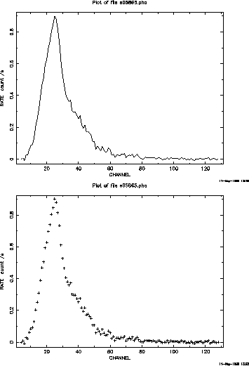
  fplot: is a very useful environment, allowing you to make simple plots of the FITS files you have. After typing fplot, you are prompted for the file name and names of two columns you would like to plot (use flcol to get these column names before using fplot). It then asks for some row range, output type and plot command, which you can keep as defaults for now.

  Figure: Example of Gk Per spectrum, with marker off (top panel) and marker on (bottom panel)

  

  You'll reproduce the top half of figure 3 if you use flcol on the rate and channel columns of s05865.pha (an energy spectrum of gk per) while keeping the marker off. Adding markers gives you the bottom half of figure 3.

  Notice also the PLT$>$ prompt. This is the plotting environment which leaves you in charge of the data you want to see. The following commands will help quite a bit in this environment:

  • help: you can guess what it does. Once you get the help$>$ prompt, you type the command you want to know about. CONTROL-D gets you back to PLT$>$.
  • plot gives you either a line or scatter plot.
  • marker off/on switches from line to scatter plot.
  • marker size N on changes the marker size to N where N is a real number from 1.0 to 5.0, probably points.
  • marker Z on switches to a specific marker type. Z goes from 1 to at least 16.
  • rescale x xmin xmax rescales the plot to zoom in on a part of your data set. FPLOT plots the entire data set by default. So use rescale to fix this. The plot is automatically updated after rescaling.
  • hardcopy /ps makes a Postscript hardcopy of the current plot. Very useful.
  • device [device] Sends the output to specified device. The device can usually be either /xw or /ps. This is useful if you want to switch from screen to hardcopy in the middle of an analysis.

  So, moving back to that gk per plot, note that we now have the tools to examine the data in more detail and to make more sophisticated plots. Write at the PLT$>$ prompt, marker on, hit enter, and then, marker size 5.0 on. This plots each datum with a cross, of 5.0 pt. Typing plot gives you the same plot, but with discrete data this time, so you can get a much better idea of the errors on your data. By default, fplot places labels on your plot. These labels are nothing more than the output from flcol.

  $\circ$ Exercise 1: Use flcol and fplot to make a scatter plot of the file s05479.pha. This is actually an EXOSAT ME spectrum of the source AM Her (sequence number 85), so it is a good idea to plot CHANNEL vs. RATE. This file is located in the directory /home/vastro/tutorial/ftools. Also note that you will be using slightly different files, like the one in the example above. Use triangular markers (yes, you will have to experiment to find these markers).

  Challenge: Learn about adding your own labels to plots and then relabel the x-axis in (angstroms).

  Figure: Gk Per light curve and power spectrum.