Keldysh Version of Iterative Perturbation Theory at Half Filling

Introduction

So far finite temperature calculations with the ordinary IPT scheme have mostly been done using the Matsubara frequency dependent Green functions [1]. It turns out that on the imaginary axis convergence is achieved quickly. However, in order to obtain the density of states one has to continue the numerical values of $G(i\omega_n)$ to the real axis which requires more sophisticated tools (e. g. the maximum entropy method) [2].

Here we will describe how iterative perturbation theory (at half filling) can be formulated in real frequency space using the Keldysh formalism. Thus, an elegant way of computing the density of states at finite temperatures is provided.

Formalism

The Keldysh formalism [3] is a generalization of the standard $T=0$ diagram technique to finite temperatures. It uses four different Green functions ($G^{--}$, $G^{++}$, $G^{+-}$ and $G^{-+}$) which for fermions are defined as follows:

$$iG^{--}(x_1,t_1;x_2,t_2) := \langle T \psi(x_1,t_1) \psi^+(x_2,t_2) \rangle$$

$$= \theta(t_1-t_2) \langle \psi(x_1,t_1) \psi^+(x_2,t_2) \rangle - \nolinebreak$$

$$\theta(t_2-t_1) \langle \psi^+(x_2,t_2) \psi(x_1,t_1) \rangle$$ (1)

$$iG^{++}(x_1,t_1;x_2,t_2) := \langle \tilde T \psi(x_1,t_1) \psi^+(x_2,t_2) \rangle$$

$$= \theta(t_2-t_1) \langle \psi^+(x_1,t_1) \psi(x_2,t_2) \rangle -$$

$$\theta(t_1-t_2) \langle \psi(x_2,t_2) \psi^+(x_1,t_1)$$ (2)

$$iG^{+-}(x_1,t_1;x_2,t_2) := \langle \psi(x_1,t_1) \psi^+(x_2,t_2) \rangle$$ (3)

$$iG^{+-}(x_1,t_1;x_2,t_2) := \langle \psi^+(x_2,t_2) \psi(x_1,t_1) \rangle$$ (4)

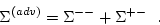
It is easy to verify that

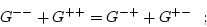$$G^{--} + G^{++} = G^{-+} +G^{+-} \mbox{\ \ ;}$$ (5)

i. e. only three of these four functions are independent of each other. The advanced Green function can be obtained from

$$iG^{(adv)}(x_1,t_1;x_2,t_2) := -\theta (t_2-t_1) \langle \psi(x_1,t_1) \psi^+(x_2,t_2)+ \psi^+(x_1,t_1)\psi(x_2,t_2)\rangle$$

$$= G^{--}- G^{+-}$$

$$= G^{-+}- G^{++}\mbox{\ \ .}$$ (6)

A similar relation holds for $G^{(ret)}$.

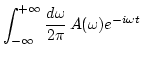
For noninteracting fermions the Fourier transforms of (1) to (4) are given by

$$G^{(0)^{-+}}(\omega,p) = 2\pi i \, \,n_p\,\delta(\omega-\epsilon_p+\mu)$$ (7)

$$G^{(0)^{+-}}(\omega,p) = -2\pi i\, \,(1-n_p)\,\,\delta(\omega-\epsilon_p+\mu)$$ (8)

$$G^{(0)^{--}}(\omega,p) = \frac{1-n_p}{\omega-\epsilon_p+\mu+i 0^+}\, + \, \frac{n_p}{\omega-\epsilon_p+\mu-i 0^+}$$ (9)

$$G^{(0)^{++}}(\omega,p) = -\left(G^{(0)^{--}}(\omega,p)\right)^*$$ (10)

where $n_p$ denotes the Fermi factor.

In the corresponding diagram technique each vertex has a $+$ or $-$ sign so that there are four contributions to the self energy: $\Sigma^{++}$, $\Sigma ^{--}$, $\Sigma^{-+}$ and $\Sigma ^{+-}$. Again only three of them are independent since

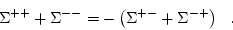$$\Sigma^{++}+\Sigma^{--}= - \left(\Sigma^{+-}+ \Sigma^{-+} \right) \mbox{\ \ .}$$ (11)

The advanced self energy can be obtained by

$$\Sigma^{(adv)} = \Sigma^{--}+ \Sigma^{+-} \mbox{\ \ .}$$ (12)

Within this framework iterative perturbation theory can be performed in the following way:

We start with a guess for the advanced Green function $G^{(adv)}(\omega)$. Then $G^{adv}_0(\omega)$ is determined by:

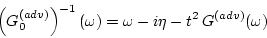$$\left(G_0^{(adv)}\right)^{-1}(\omega) = \omega- i\eta-t^2\,G^{(adv)}(\omega)$$ (13)

Let $A(\omega)$ be the spectral weight of $G^{(adv)}_0$:

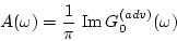$$A(\omega)=\frac{1}{\pi}\,\, \mbox{Im}\, G^{(adv)}_0 (\omega)$$ (14)

It is convenient to introduce functions $A(t)$ and $\tilde{A}(t)$ as Fourier transforms of $A(\omega)$ and $\tilde{A}(\omega):= A(\omega) \, n_f(\omega)$:¹

$$A(t) = \int_{-\infty}^{+\infty} \frac{d\omega}{2\pi}\,A(\omega) e^{-i\omega t}$$ (15)

$$\tilde{A}(t) = \int_{-\infty}^{+\infty} \frac{d\omega}{2\pi}\, \tilde{A}(\omega) e^{-i\omega t}$$ (16)

Now, using $G^{\sigma \sigma}= \int d\epsilon_p \, G^{(0)^{\sigma \sigma}}(\omega,\epsilon_p)\,\, A(\epsilon_p)$, and (7) to (10), we can express all four Green functions in terms of $A(t)$ and $\tilde{A}(t)$:

$$G^{--}_0(t) = 2\pi i\, \left( -\theta(t) \left(A(t)-\tilde{A}(t)\right) + \theta(-t) \tilde{A}(t)\right)$$

$$G^{++}_0(t) = \left(-G^{--}_0(-t)\right)^{\star}$$

$$G^{-+}_0(t) = 2\pi i\, \tilde{A}(t)$$

$$G^{+-}_0(t) = -2\pi i\, \left(A(t) - \tilde{A}(t) \right)$$ (17)

These Green functions are necessary to evaluate the second order self energy diagrams for $\Sigma ^{--}$ and $\Sigma ^{+-}$ (see figure 1):

Figure 1: Second order diagrams for $\Sigma ^{--}$ and $\Sigma ^{+-}$

$$\Sigma^{--}(t) = U^2\, \left( G_0^{--}(t) \right)^2 G_0^{--}(-t)$$

$$\Sigma^{+-}(t) = -U^2\, \left( G_0^{+-}(t) \right)^2 G_0^{-+}(-t)$$ (18)

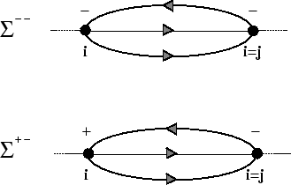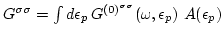
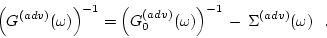
Now equations (6) and (12) allow us to change back to the advanced functions:

$$G_0^{(adv)}(t) = G_0^{--}(t) -G_0^{+-}(t)$$

$$\Sigma^{(adv)}(t) = \Sigma^{--}(t)+\Sigma^{+-}(t)$$ (19)

The new (full) Green function $G^{(adv)}$ is finally given by

$$\left(G^{(adv)}(\omega)\right)^{-1}= \left(G_0^{(adv)}(\omega)\right)^{-1} \, - \, \Sigma^{(adv)}(\omega) \mbox{\ \ .}$$ (20)

Returning to equation (13) closes the iteration.

The numerical implementation requires Fourier transforms between time and frequency space. These can be realized by using fast Fourier transforms.

We formulated the equations for the Hubbard model. The corresponding results will be presented in the next section. But this procedure can also be applied to the large $d$ limit of other lattice models. In most cases only slight modifications are necessary.