Introduction to simulation method
Per Stoltze
Center for Atomic-scale Materials Physics
Department of Physics, Building 307,
DK-2800 Lyngby
Simulations
combine an interaction potential with a
numerical solution of the equation of motion
followed by statistical treatment of the results.
The main purpose of the simulation is insight, not data.
Even if simulations may contribute to both theory and experiments,
the most important result of simulations is undoubtedly the
development of intuition and ideas through interactive simulations.
Limitations of simulation
The first limitation of simulations is that
agreement between the simulation and the behavior of the real system
at the macroscopic level proves nothing about
the simulation at the microscopic level.
Assessment of the realism of simulation requires an insight which
transcends the simulation.
The second limitation of simulations is that simulations are not
persuasive.
We may believe the
microscopic model and we may trust the correctness of the software.
Once the simulation starts, the atoms move under their
mutual interaction, and the situation becomes much to
complex to be followed mentally.
A sceptic can always choose to believe that the microscopic
model is incorrect, the software is buggy or the statistics is insufficient.
The third limitation of simulations is that the insight, which is the
purpose of the simulation, is far from being automatic.
If we cannot find a simple macroscopic model, the data generated in the
simulation may forever remain just data.
The interaction potential
The interaction potential used in the simulation
may be generic or realistic.
A generic potential
attempts to capture the essential
physics while the structure of the potential is simplified as much as
possible.
Generic potentials are used to study phenomena and models.
A realistic potential attempts to describe real materials under
specific conditions.
Realistic potentials may be either accurate or approximative.
From a simulation point of view, the approximate total energy methods
are interpolation schemes used to calculate the energy from
parameters derived from experiments or from first principle calculations.
At the simplest level, the interaction potential consists of a sum
of pair-wise interaction energies.
At the intermediate level, the energy for the system consists of
a sum of energies for the atoms, but the energy cannot be
decomposed into a sum of pair-wise interaction energies.
For the quantum case, the energy of the system cannot be decomposed
into a sum of pair-wise interaction energies or even as a sum of
energies for the individual atoms.
The principles and implementation of the simulation methods are almost
independent of the interaction potential used.
However, if the potential happens to be a pair-potential and the
implementation exploits this, then is almost impossible
to adapt the program to use a non-pair-potential.
Careful analysis is needed to discover the implicit assumption
of pair-wise interactions e.g. in the layout of loops.
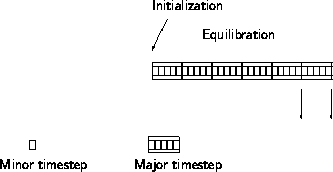
The principle in a simulation.
At the initialization, a configuration is generated or read from a file.
The system is then equilibrated by propagation in time.
When the system has equilibrated, the production phase starts.
Data are stored on disk when the production phase starts and then
after each major timestep.
The major timestep is an abstraction.
Frequently the major timestep is too long for the simulation method
and the program internally builds up the major timesteps through a series
of minor timesteps.
Stochastic and deterministic simulations
Simulations are either stochastic or deterministic, depending
on the nature of the equation of motion used in the simulation.
For the stochastic methods
the equation of motion is artificial
and tries to generate configurations with certain statistical properties.
Average data are calculated as ensemble averages

Monte Carlo is the most important of the stochastic techniques.
Deterministic methods
aim at observation of the evolution in time of
the system.
This is usually done by numerical solution of the equation of motion.
Average data are calculated as a time average

over the trajectory.
Some elements of randomness are often introduced in the purely deterministic
methods to improve the approach to thermodynamic equilibrium and
to increase the temperature control.
Molecular Dynamics is the most important of the deterministic techniques.
Phases in a simulation
A simulation consists of 3 phases:
initialization, equilibration and production.
In the initialization
the positions and momenta of the atoms
are generated or loaded from a previous simulation.
During the equilibration
the simulation is run until
equilibrium is reached and the memory of the initial configuration
has been erased.
In simulations of kinetic phenomena, this phase is omitted.
If the initial configuration is far from equilibrium, one may reach
a good estimate for the equilibrium properties if the initial, atypical
configurations are discarded.
During the production phase
the simulation is continued while
data are stored on disk or analyzed concurrently with the simulation.
The results are extracted from the simulation by
direct computation of structural data from the final configuration,
by extraction of thermodynamic or kinetic data by statistical treatment
of the collected data, or
by visualization and animation.
Program design
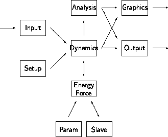
Modules in a simulation program. Arrows indicate flow of information.
The setup, simulation, graphics, and analysis
are usualy distributed over a number of programs.
Each of the programs consists of a number of modules.
The main modules in a simulation program are illustrated in figure
\ref{fig:simmodul}.
The initialization of the simulation is made by loading data from
a previous simulation through the input module or by generation
of a new configuration in the setup module.
The total energy method used as the basis for the simulation is
implemented in the energy module.
The parameters may be loaded from a database or
the total energy method may be presented to the simulation
program in the form of a slave program.
The simulation module contains a spectrum of methods
for numerical solution of the equation of motion.
As simulations may consume enormous computational resources it is
important that the program provides an analysis module for
use while the simulation is in progress.
The analysis module should contain
facilities for a preliminary analysis of the results
as well as a facility for detailled
analysis of the performance of the simulation algorithm.
The output from a simulation program is primarily data for further analysis by
other programs. The data may also form the starting point for further
simulations.
Images and graphs stored during the simulation may also be an efficient
way of reviewing the simulations. It is convenient to
review the progress of extended simulations by replaying the stored
images as animations every few hours while the simulation is in progress.
Random Numbers
Random numbers are an important ingredient of stochastic simulation
algorithms.
A sequence of pseudo-random numbers are
generated using a reproducible, deterministic algorithm.
The essential property of this algorithm
is that the numbers have the same statistical properties as
independent, identically distributed numbers.
A linear congruental generator
has the transition function

where m is the modulus,
a is the multiplier,
1<a<m,
c is the increment,
 , and
, and
 indicates the remainder
when y is divided by x.
The states are the integers
0
  sn < m
for c>0 and
1
  sn < m for c=0.
s is normalized to a floating point number in the interval [0,1[
by floating point division, s/m.
The advantages of the linear congruental generators are that they have
high speed and use a minimum of memory.
They are reproducible and portable.
The quality of the generated numbers is analyzed by numerical
and number theoretic methods.
The minimal standard
is the generator a=16807 c=0 and m=2^{31}-1=2147483647
Periodic boundary conditions
We will write the positions of atoms as

where C is the basis for the system,  is the real space
position, and
  +
+ is the scaled space position.
The reason for writing the scaled space position as a sum of two components
will become clear in a moment.
For atoms in the principal box, the components of
 are
0
are
0  si < 1, i=1,2,3.
Scaled coordinates are used inside the program.
If necessary, the conversion to and from scaled coordinates
is made in the input and output function.
The advantage of scaled coordinates is that the treatment of periodic
boundary conditions in scaled space is straight-forward.
In the presence of 3D periodic boundary conditions, we can generate
all the interatomic vectors from atom number i
and all the images of j under the translational symmetry
to atom number j by

where n1,n2,n3 = 0,
 1,
1,  2, ...
Except for very small systems or very long ranged interactions
n1,
n2, and
n3 may be limited to the values -1,0,1.
The absence of periodic boundary conditions is implemented by
restriction of the values for (n1,n2,n3) to (0,0,0).
For cases where the interactions are long ranged compared to the
size of the system, the interaction of an atom
with its own images under the translational symmetry
may contribute significantly to the total energy.
For symmetry reasons there is no corresponding force.
Under
the minimum image convention
the statement that i and j are
neighbors indicate that only the shortest of the vectors in Equation
\ref{eq:pbcbf} should be included in the computation.
This vector can be projected out very efficiently and the
periodic boundary conditions may be encapsulated in a few lines
of code, here in the two if-statements:
\label{sc:mic}
int   i1, i2;
double rs[3], rd[3];

for (i1 = 0; i1 < 3; i1++)
 rs[i1] = atom[ic].spos[i1] + atom[ic].dpos[i1]
          - atom[io].spos[i1] - atom[io].dpos[i1];

if (symmetry == 1 || symmetry == 3)
{
 rs[2] -= (rs[2] > 0.) ? (int) (rs[2] + 0.5) : (int) (rs[2] - 0.5);
}
if (symmetry == 2 || symmetry == 3)
{
 rs[0] -= (rs[0] > 0.) ? (int) (rs[0] + 0.5) : (int) (rs[0] - 0.5);
 rs[1] -= (rs[1] > 0.) ? (int) (rs[1] + 0.5) : (int) (rs[1] - 0.5);
}
for (i1 = 0; i1 < 3; i1++)
{
rd[i1] = 0.;
for (i2 = 0; i2 < 3; i2++)
rd[i1] += cbdir[i1][i2] * rs[i2];
}
\end{verbatim}
Here the vector atom[ic].spos is the scaled space position for
atom number ic,
cbdir is the basis,
rs and rd are the interatomic vector in scaled and real
space, respectively.
symmetry~=~1 corresponds to periodic boundary conditions along the
third basis vector,
symmetry~=~2 to periodic boundary conditions along the two first
basis vectors, and symmetry~=~3 to periodic boundary conditions
along all three basis vectors.
Implicit in this implementation is
the absence of assumptions on the orientation of the basis in real
space. E.g. if symmetry~=~1 the direction of the symmetry axis can
be made to coincide with any direction in space, including the x,
y, or z-axis, by a rotational transformation of the
components of cbdir.
Neighbor lists
Even for relatively small systems, it will pay off to maintain
a list of the significant interactions: the neighbor list.
The calculation of force or energy can then be made much faster
by neglecting the insignificant interactions.
The lists are allocated when the atom array is allocated.
Using the same length for the neighbor list for all atoms allow the
lists to be allocated as one block of memory.
Allocating the lists individually and reallocating the lists as they
grow leads to an unacceptable fragmentation of memory.
The list for each atom contains an array of pointers to the neighbors.
This is more elegant and slightly more efficient than using an array of
the indices of the neighbors.
The scaled positions are split into two contributions

where  is the scaled space position at the most recent update
of the neighbor list and
 is the displacement of the atom since the last update.
The displacements of the atoms are checked after each step in the simulation and
the lists are updated when required.
Depending on the details of the program,
one may decide to include each
neighbor pair on the neighbor lists of one or both of the atoms
in the pair.
\label{alg:listhalf}
If the atoms i and j, with j<i, are neighbors and j is a
member of the neighbor list for i, but i is not a member of
the list for j, we will say that the program uses a half-list.
\label{alg:listfull}
If i is a member of the neighbor list for j and vice versa
we will say that the program uses a full-list.
Both for half-lists and for full-lists it may be advantageous to keep
the lists sorted.
If the program only needs to loop over pairs of atoms, the use of a half-list
is more efficient. However, if the program ever needs to loop over
neighbors of a particular atom, the use of a full-list is more
efficient.
Fortunately, if the lists are kept sorted
a half-list can easily be folded into a full-list
and a loop over pairs can easily be made immune to the use of half- or
full-lists
\begin{verbatim}
int ic, in;
struct ATOM *nbr;
for(ic=0; ic
here natoms is the number of atoms,
atom[ic].nbrgs is the number of neighbors for atom number ic,
the array atom[ic].nbr stores the pointers to the neighbor atoms.
This device is used, if possible, in all functions.
It is then easy to switch the entire program
between the use of full-lists or half-lists.
Static atoms
Static atoms can eliminate some the problems caused by the presence
of free surfaces.
Static atoms take part in the energy and force calculations
but do not move during the simulation.
The atoms are loaded into the atom array in a specific sequence,
figure \ref{pic:atomSeq}.
The first n1 atoms are static
and do not participate in the dynamics.
The next n2-n1 atoms in the atom struct
are dynamic and active and the rest of the atoms are inactive.
The inactive atoms are necessary for the implementation of growth.

Storage of atoms in the atom array.
0, n1, and n2 indicates the first atom, the first dynamic atom and
the first inactive atom, respectively.
\label{pic:atomSeq}}
\end{figure}
Force and energy calculations loop over the active atoms,
the dynamics functions loop over the dynamic atoms, and the
output function prints data for all atoms.
Growth
The atoms to be grown during the simulation are allocated as
inactive atoms at the startup of the simulation.
Growth is then simulated by activating these atoms sequentially during
the simulation.
Constraints
During the simulation it is useful to be able to constrain a single atom
or a group of atoms to move in a particular direction with a constant
speed, while all other degrees of freedom take part in the simulation.
This requires that two degrees of freedom orthogonal to the constraint
direction are constructed for all constrained atoms and that these
degrees of freedom are included in the simulation.
At the beginning of each major timestep the constrained atoms are
moved the appropriate distance along the direction of the
constraint.
During the major timestep, the constrained atoms only move orthogonal to
the direction of the constraint.
For Molecular Dynamics
the implementation of the constraints
amounts to removing the component of the force parallel with the direction
of the constraint.
For Monte Carlo
the random move is generated as usual, but
the unwanted component of the move is eliminated before proceeding with the
evaluation of the move.
\label{impl:cnstrn}
The constraints are implemented through a table of constraints.
Each atom has a pointer, cnsvec, to a constraint vector
For constrainted atoms cbsvec points to an entry in a
constraint table.
For unconstrained atoms cnsvec is a null-pointer.
Models
Different models may be used to represent the atomic structure of
the system.
The models are important because the choise of model has implications for
both the data structure and the simulation methods.
Particle models use a description in terms of atoms moving as
point masses in space.
The identity of each atom is fixed and
the dynamics consists of the atoms moving subject to the interatomic
forces.
For particle models, the interatomic distance is a continuous variable and
cannot be tabulated. Consequently, the computational efficiency is lower
than for a grid model.
The computation of interactions are made through dynamically updated neighbor
lists.
In a particle model vacancies are not explicitly represented,
their number is not conserved,
and their positions are generally hard to determine.
Grid models use a description in terms of atoms and vacancies
occupying the sites of a regular grid.
The dynamics consist of atoms changing their identity or of atoms
moving from one site to another.
As the atoms can only occupy the sites of the grid, there are no forces,
and deterministic simulation is difficult.
Computations for grid models are faster than for particle models.
The neighbor lists
are static and may be determined during
startup of the simulation or hardcoded in the layout of arrays.
The interactions are easily tabulated.
In a grid model vacancies are included explicitely,
and the structure and
dynamics of vacancies may be studied by exactly the same methods as
for the atoms.
However, a vacancy occupies as much memory as an atom.
Energy minimization
Steepest descent is used to find the minimum energy configuration.
The principle is to perform the energy minimization through
repeated minimizations along the direction of the force.
Given the force,  , a step length, c, and a fraction, u, of this
step length

If we assume that

is locally parabolic

The minimum is

It is obvious that steepest descent may converge to a stationary point, which is
not a minimum. As the potential energy surface frequently has
numerous local minima, it requires some insight and a bit of luck to
make steepest descent converge to the global minimum.
Monte Carlo algorithms
The significant contribution to the phase-space average,
<A>, Equation \ref{eq:ensAver},
comes from the
parts of phase-space where the energy,  is close to its minimum,
the exponential function
suppresses the contributions from regions of higher energy.
The principle behind the Monte Carlo algorithm
is to
rewrite Equation \ref{eq:ensAver} as

to show that the average is calculated by integration over all of phase-space,
i.e. each point in phase-space is included with probability 1,
and weight

The idea due to Metropolis et al.
is to swap the interpretations of weight and probability:
Configurations are included with weight 1
and probability

In the Monte Carlo algorithm
random moves are generated and accepted or rejected with
appropriate probability.
There are several options for the random moves.
Atoms may be moved randomly relatively to their present configuration and
an attempted move may involve one or more atoms.
One may loop through the atoms sequentially or in random order.
When an attempted move has been generated, the neighbor list must
be checked and, if necessary, updated before the energy is calculated.
If the attempted move is rejected, the atoms must be moved back,
the previous size and shape of the box must
be restored, and the lists checked again.
The starting point is the probability,
 of observing some state i.
In a discrete model

where the transition probability

from
 to
to
 is arbitrary except that it satisfies detailed balance.
As we want the algorithm to establish the canonical contribution
the transition probability should satisfy the equation

This is not enough to determine
 and
there are families of Monte Carlo algorithms corresponding to various
functional forms for

The average of some property, A, may be calculated as the arithmetic
mean from the configurations,
Am, m=1,...,M, generated by the
Metropolis algorithm

Monte Carlo simulations use large quantities of random numbers and
the quality of the random number generator
is important for the quality of the calculated results.
The Metropolis algorithm for the (NTV) ensemble
Metropolis et al. defined

for the transition probability,
 Equation \ref{eq:canonw}.
C is an arbitrary constant, C>0.
It is important that the implementation of the Metropolis algorithm
is stable against overflow of the exponential function and against
division by zero for T=0. This may be done by splitting the
test

into 3 steps
if( delene < 0. ||
  (delene < 15.*kbt && exp(-delene/kbt) > ran()))
     accept();
  else
     reject();
where delene is  and
kbt is kBT.
The first test shortcuts the case where

the second test first checks for

and then checks the exponential function against a random number.
The second test has been implemented, so that T=0 does not require
special treatment.
The Glauber algorithm for the (NTV) ensemble
In the Glauber algorithm
the transition probability is

The Metropolis algorithm for the (NTp) ensemble
If we assume that the Hamiltonian is separable
when the volume is changed

the transition probability for the (NTp) ensemble is

Kinetic Monte Carlo
Kinetic Monte Carlo is based on
Equation \ref{eq:masterEq}.
When the system is in some state,
 , the transition rate out of
this state is

The time spent in state
 is chosen as

where u is a random number uniform in ]0,1].
 is chosen as the new state with probability

The main advantages of kinetic Monte Carlo is that time is well-defined
and only a small number of elementary reactions are considered.
Experiments or
Molecular Dynamics simulations are often used to determine the
parameters for a kinetic Monte Carlo simulation.
Microcanonical Monte Carlo
Ray has derived a micro-canonical Monte Carlo
algorithm starting from the transition probability

where

where c is a constant.
Evidently, the energy,
 ,
of the initial configuration must not
exceed E.
When this requirement is satisfied for the initial configuration, the
algorithm guarantees that
 for all i
  0 .
0 .
Molecular Dynamics
The principle in Molecular Dynamics
is the numerical integration of
the classical equation of motion in Lagrangian or Hamiltonian form,
In the numerical solution, the immediate results are the
positions, momenta, forces, and various components of the energy.
Other data, such as thermodynamic averages, order parameters, and
spectra are calculated later from these data.
The maximum usable timestep
is limited by the stability of the numerical algorithm.
This complicates the study of slow phenomena and rare events.
The velocity-Verlet algorithm is

The integration can be implemented without additional storage
by overlaying
 ,
,
 and
and
 ,
overlaying
 ,
and
,
and
 and overlaying
 and
and

\begin{verbatim}
for(im=0; im
if (chkList() != 0 || force() != 0)
return 1;
for (ic = natoms[0]; ic < natoms[1]; ic++)
for (i = 0; i < 3; i++)
atom[ic].smom[i] += 0.5 * atom[ic].sfrc[i] * mdtime;
}
\end{verbatim}
Provided that
 and
and
 are used as initial conditions and
 is calculated as part of the startup
procedure, the velocity-Verlet algorithm is self-starting.
Control of temperature
As Molecular Dynamics algorithms conserve the
total energy on average,
it is difficult to guess the initial conditions which
will eventually establish the desired temperature.
We thus need a mechanism which will establish a desired
temperature during the initial part of a simulation when the final
part of the simulation is to be performed micro-canonically.
A temperature may be established by periodically rescaling the
momenta to the desired temperature.
In stochastic thermalization atoms are selected
randomly and assigned a new momentum drawn from a Boltzmann distribution
corresponding to the desired temperature.
The Boltzmann distributed momenta are easily generated by the Box-M\"uller
algorithm.
Berendsen thermalization
may be combined with most integration methods by
rescaling of the momenta
at the start of each major timestep:

where h is the length of the major timestep,
 is the desired relaxation time for the temperature,
and
T0 is the desired temperature.
Control of pressure
The integration algorithms discussed so far all work at a constant
volume.
The pressure may be kept constant by optimization of
the volume of the box at the start
of each major move during the equilibration.
In Berendsens algorithm the volume is rescaled at the start of each
major timestep

This algorithm is analogous to the Berendsen algorithm for temperature
control and these two algorithms may be combined.
Abrahams method for pressure control consists of
a combination of Monte Carlo for the box with Molecular Dynamics for the
atoms.
At the start of each major move,
one attempted Monte Carlo move is made for the box using
constant pressure Monte Carlo dynamic.
Molecular Dynamics at constant temperature
One possible starting point for the derivation of an isothermal
Molecular Dynamics algorithm is the Langevin equation of motion:

where
 is the force from the surrounding atom and R(t) is a stochastic
force

One possible algorithm is
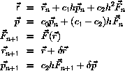
where

 and
and
 are temporary variables, and
 and
and
 are stochastic components
with zero mean and specified variance and correlation .
Molecular dynamics at constant p and T
The Andersen algorith uses scaling of V to control
the pressure.
The equation of motion is

where p is the instantaneous pressure and
 is the desired
pressure.
The equation of motion is integrated as
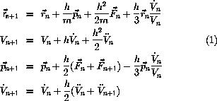
The inertia, Q, for the box is not important for the
calculated equilibrium properties.
Creutz Demon
The idea of the Creutz Demon algorithm is to introduce
an additional degree of freedom in the system.
This extra degree of freedom is called the demon.
The energy is
E=Ec + ED,
where Ec is the energy of the system and
ED is the energy of
the demon.
ED is adjusted to keep E constant
through the following algorithm:
- The system has energy Ec and the demon
has energy ED.
- Generate an attempted change and calculate the energy change,
 .
for the system.
- If
 the new configuration is accepted and
 is subtracted from ED.
If
 the attempted move is rejected and the old
configuration is restored.
The Creutz Demon algorithm contains both
the canonical and the micro-canonical averages as
limiting cases and is capable of interpolating between these two
limits.
The generalization to use many demons is straight-forward.
The algorithm will simulate
a micro-canonical ensemble with 3N+n degrees of freedom
and, at least for large values of n,
a canonical ensemble of N degrees of freedom.
Suggested reading
F. F. Abraham:
Computational statistical mechanics: Methodology applications and
supercomputing. Adv. Phys. 35 (1986) 1.
M. P. Allen and D. J. Tildesley:
Computer simulation of liquids.
Clarendon Press, Oxford (1987).
H. C. Andersen:
Molecular dynamics simulations of constante pressure and/or temperature.
J. Phys. Chem. 72 (1980) 2384.
E. Atlee Jackson:
Perspectives of nonlinear dynamics. Volume I \& II.
Cambridge University Press, Cambridge,
(1991).
H. J. C. Berendsen, J. P. M. Postma, W. F. van Gunsteren,
A. DiNola, and J. R. Haak:
Molecular dynamics with coupling to an external bath.
J. Chem. Phys. 81 (1984) 3684.
G. Bhanot:
The Metropolis algorithm.
Rep. Prog. Phys 51 (1988) 429.
K. Binder:
Monte Carlo methods in statistical physics.
2nd edition.
Topics in current physics
volume 7,
Springer Verlag, Berlin (1986).
K. Binder:
Application of the Monte Carlo method.
2nd edition.
Topics in current physics,
volume 36,
Springer Verlag, Berlin (1987).
J. Q. Broughton, G. H. Gilmer, and J. D. Weeks:
Constant pressure molecular dynamics simulations of the 2D
r-12 system: Comparison with isochores and isotherms.
J. Chem. Phys. 75 (1981) 5128.
D. Chandler:
Introduction to modern statistical mechanic.
Oxford University Press, Oxford (1987).
M. Creutz:
Microcanonical Monte Carlo simulation.
Phys. Rev. Lett. 50 (1983) 1411.
B. W. Dodson and P. A. Taylor:
Monte Carlo simulation of continuous-space crystal growth.
Phys. Rev. B 34 (1986) 2112.
P. L'Ecuyer: Random numbers for simulation.
Commun. ACM 33 (1990) 85.
J. D. Foley, A. van Dam, S. K. Feiner, and J. F. Hughes:
Computer Graphics., 2nd edition.
Addison-Wesley Publishing Co. Massachusets (1990).
J. R. Fox and H. C. Andersen:
Molecular dynamics simulations of a supercooled monoatomic liquid and
glass.
J. Phys. Chem. 88 (1984) 4019.
H. Gould and J. Tobochnik:
An introduction to computer simulation methods. Volume 1+2.
Addison-Wesley Publishing Co. Massachusetts
(1988).
D. W. Heermann:
Computer simulation methods.
Springer Verlag, Berlin (1986).
R. W. Hockney and J. Eastwood:
Computer simulation using particles.
Adam Hilger, Bristol (1988).
Wm. G. Hoover:
Molecular Dynamics.
Lecture Notes in Physics volume 258 (1986).
J. D. Lambert:
Numerical methods for ordinary differential systems.
John Wiley \& Sons, Chichester.
(1991).
N. Metropolis, A. W. Rosenbluth, M. N. Rosenbluth, A. H.
Teller, and E. Teller:
Equation of state calculations by fast computing machines.
J. Chem. Phys. 21 (1953) 1087.
J. F. Nicholas:
Some ball models of crystals and crystal surfaces.
J. Phys. Chem. Solids 23 (1962) 1007.
S. K. Park and K. W. Miller:
Random Number generators: Good ones are hard to find.
ACM Commun. 31, (1988) 1192.
W. H. Press, B. P. Flannery, S. A. Teukolsky, and W. T. Vetterling:
Numerical Recipes in C.
Cambridge University Press, Cambridge (1988).
A. Rahman:
Correlations in the motion of atoms in liquid argon.
Phys. Rev. 136 (1964) A405.
J. R. Ray:
Microcanonical ensemble Monte Carlo metod.
Phys. Rev. A 44 (1991) 4061.
M. J. Rochkind:
Advanced Unix programming.
Prentice Hall International Inc., New Jersey (1985).
S. K. Schiferl and D. C. Wallace:
Statistical errors in molecular dynamics averages.
J. Chem. Phys. 83 (1985) 5203.
R. Sedgewick:
Algorithms in C.
Addison-Wesley Publishing Co. Massachusets (1990).
P. Stoltze:
Simulation methods in atomic-scale materials physics.
Polyteknisk Forlag, Lyngby (1997).
W. C. Swope, H. C. Andersen, P. H. Berens and K. R. Wilson:
A computer simulation method for the calculation of equilibrium constants
for the formation of physical clusters of molecules: Application to
small water clusters.
J. Chem. Phys. 76 (1982) 637.
L. Verlet:
Computer experiments on classical fluids. I. Thermodynamical
properites of Lennard-Jones molecules.
Phys. Rev. 159 (1967) 98.
A. F. Voter:
Classically exact overlayer dynamics: Diffusion of rhodium
clusters on Rh(100).
Phys. Rev. B 34 (1986) 6819.
W. W. Wood and F. R. Parker:
Monte Carlo equation of state of molecules interacting with the
Lennard-Jones potential. I. A supercritical isoterm at about twice the
critical temperature.
J. Chem. Phys 27 (1957) 720.


 , and
, and
 indicates the remainder
when y is divided by x.
The states are the integers
0
  sn < m
for c>0 and
1
 is the real space
position, and
  +
+ is the scaled space position.
The reason for writing the scaled space position as a sum of two components
will become clear in a moment.

 1,
1, 

 , a step length, c, and a fraction, u, of this
step length


 is close to its minimum,
the exponential function
suppresses the contributions from regions of higher energy.


 of observing some state i.
In a discrete model


 to
to
 is arbitrary except that it satisfies detailed balance.

 and
there are families of Monte Carlo algorithms corresponding to various
functional forms for


 Equation \ref{eq:canonw}.
C is an arbitrary constant, C>0.

 and
kbt is kBT.


 , the transition rate out of
this state is

 is chosen as

 is chosen as the new state with probability


 ,
of the initial configuration must not
exceed E.
When this requirement is satisfied for the initial configuration, the
algorithm guarantees that
 for all i
  0 .
0 .

 ,
,
 and
and
 ,
overlaying
 ,
and
,
and
 and overlaying
 and
and

 and
and
 are used as initial conditions and
 is calculated as part of the startup
procedure, the velocity-Verlet algorithm is self-starting.

 is the desired relaxation time for the temperature,
and
T0 is the desired temperature.


 and
and
 are stochastic components
with zero mean and specified variance and correlation .

 is the desired
pressure.

 .
for the system.
 the new configuration is accepted and
 is subtracted from ED.
If
 the attempted move is rejected and the old
configuration is restored.