Measurement Error Propagation
Here, we are interested in estimating the error of our result, provided we know the error of input variables. In experiments, measurements are always known only up to finite precision. It is important to quantify the resulting uncertainty before we can reliably interpret the results of the measurement.
Suppose that we want to calculate error estimation of function $f(x,y)$, where both $x$ and $y$ are known with finite precision. We either have a large number of measurements of $x$ and $y$, or, we might know the probability distribution of measurements and their averages. For now, let's assume
For now, let's assume that we have measured $x$ and $y$ and have a large number $n$ of measurements with values $[x_0,x_1,...,x_{n-1}]$ and $[y_0,y_1,...,y_{n-1}]$. Using statistics, we can define
$$<x> = \frac{1}{n}\sum_{i=0}^{n-1} x_i$$$$<y> = \frac{1}{n}\sum_{i=0}^{n-1} y_i$$$$\sigma_x^2 = \frac{1}{n-1}\sum_{i=0}^{n-1} (x_i-<x>)^2$$$$\sigma_y^2 = \frac{1}{n-1}\sum_{i=0}^{n-1} (y_i-<y>)^2$$In many experimental measurements we can assume that errors on measurement of $x$ and $y$ are uncorrelated. On the other hand, there are cases of non-negligible correlation between the measurements of different variables. In the latter case, the covariance should also be nonzero:
$$cov(x,y)=\frac{1}{n-1}\sum_{i=0}^{n-1} (x_i-<x>)(y_i-<y>)$$$cov(x,y)$ quantifies the degree of correlation between variables $x$ and $y$.
Using the inputs $<x>$, $<y>$, $\sigma_x^2$, $\sigma_y^2$, and $cov(x,y)$, we want to estimate the error of function $f$, which we denote by $\sigma_f$. If we have $n$ measurements of $x$ and $y$, we could calculate it by
$$\sigma^2_f=\frac{1}{n-1}\sum_{i=0}^{n-1}(f_i-<f>)^2$$Below we will derive general expression for $\sigma_f$ knowing function $f(x,y)$ and the input variables and their errors.
We will work under the assumption that erros are small and can be trated in a linear approximation. If only the variable $x$ has finite error, which is small, we could estiate
$$f(x_i)-f(<x>)\approx (x_i-<x>) \frac{\partial f(<x>)}{\partial x}$$which is correct up to linear order. It then folows $$\sigma^2_f = \frac{1}{n-1}\sum_{i=0}^{n-1} (f(x_i)-f(<x>))^2= \frac{1}{n-1}\sum_{i=0}^{n-1} (x_i-<x>)^2 \left(\frac{\partial f(<x>)}{\partial x}\right)^2 = \left(\frac{\partial f(<x>)}{\partial x}\right)^2 \sigma^2_x $$
For shorter notation, we will denote the derivative $$\frac{\partial f(<x>)}{\partial x}\equiv \frac{\partial f}{\partial x}. $$ Note that we always evaluate derivative at the average value of $x$.
For single variable with uncertainty, we thus simply have
$$\sigma_f = \left|\frac{\partial f}{\partial x}\right|\sigma_x$$If the error of $y$ and $cov$ are also finite, we need to add more terms. We start by estimating
$$f(x_i,y_i)-f(<x>,<y>)\approx (x_i-<x>) \frac{\partial f}{\partial x} + (y_i-<y>)\frac{\partial f}{\partial y} + O(\Delta_x^2,\Delta_y^2,\Delta_x\Delta_y).$$Up to linear order in all variables, we have $$ \sigma_f^2=\frac{1}{n-1}\sum_{i=0}^{n-1} \left[(x_i-<x>) \frac{\partial f}{\partial x} + (y_i-<y>)\frac{\partial f}{\partial y} \right]^2 $$ which gives $$ \sigma_f^2=\sigma^2_x \left(\frac{\partial f}{\partial x}\right)^2 + \sigma^2_y \left(\frac{\partial f}{\partial y}\right)^2+2cov(x,y)\frac{\partial f}{\partial x}\frac{\partial f}{\partial y} $$
We can also write this equation in matrix form $$ \sigma_f^2 = \begin{bmatrix}\frac{\partial f}{\partial x},&\frac{\partial f}{\partial y} \end{bmatrix} \begin{bmatrix} \sigma^2_x & cov(x,y)\\ cov(x,y) & \sigma^2_y \end{bmatrix} \begin{bmatrix}\frac{\partial f}{\partial x}\\ \frac{\partial f}{\partial y} \end{bmatrix} $$
Now it is easy to generalize this equation to any number of variables $$ \sigma_f^2 = \begin{bmatrix}\frac{\partial f}{\partial x_1},&\frac{\partial f}{\partial x_2},& \frac{\partial f}{\partial x_3},... \end{bmatrix} \begin{bmatrix} \sigma^2_{x_1} & cov(x_1,x_2) & cov(x_1,x_3) & ...\\ cov(x_2,x_1) & \sigma^2_{x_2} & cov(x_2,x_3) & ...\\ cov(x_3,x_1) & cov(x_3,x_2) & \sigma^2_{x_3} & ...\\ ... \end{bmatrix} \begin{bmatrix}\frac{\partial f}{\partial x_1}\\ \frac{\partial f}{\partial x_2}\\ \frac{\partial f}{\partial x_3}\\ ... \end{bmatrix} $$
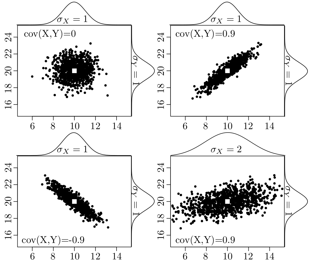
The following demonstrates covariance with a set of measurements of variables $x$ and $y$: We display 400 random measurements (black dots) which have the same means (white squares) but different covariance structures. The marginal distributions of the $x$ and $y$ variables are shown as ‘bell curves’ on the top and right axis of each plot.
Often we do not have many measurements, but we know the probability distribution of measurement $P(x)$, and we need to compute the variance from the distribution. The formulas are straighforard generalization of discrete formulas
$$\sigma_x^2 = \int dx P(x) (x-<x>)^2$$where probability is normalized $$ \int dx P(x)=1 $$ and average is given by $$<x> = \int dx P(x) x$$
We can check that with discrete probability distribution defined by $$P(x) = \frac{1}{n}\sum_{i=0}^{n-1} \delta(x-x_i)$$ we recover the discrete formulas, except that $n-1$ is replaced by $n$ in estimation of variance. For continuum distributions it is assumed that $n$ is very large, hence the two formulas are equivalent.
As an example we consider uniform distribution between $[-a,a]$. The probability is than $$P(x) = \frac{1}{2a} \theta(-a<x<a)$$ and $<x>=0$ and $$\sigma^2_x = \frac{1}{2a}\int_{-a}^a x^2 dx=\frac{a^2}{3} $$ and hence $\sigma_x = \frac{a}{\sqrt{3}}$.
As the second example we consider triangular distribution between $[-a,a]$. The probability is
$$P(x) = \frac{1}{a}\left(1-\left|\frac{x}{a}\right|\right) \theta(-a<x<a)$$This gives the average $<x>=0$ and $$\sigma^2_x = \frac{1}{a}\int_{-a}^a \left(1-\left|\frac{x}{a}\right|\right)x^2 dx=\frac{a^2}{6} $$ hence $\sigma_x = \frac{a}{\sqrt{6}}$
import numpy as np
import matplotlib.pyplot as plt

N=200
x=np.linspace(-2,2,N)
yuniform=np.hstack( (np.zeros(int(N/4)),0.5*np.ones(int(N/2)),np.zeros(int(N/4)) ))
ytriang= [0 if abs(t)>1 else 1.-abs(t) for t in x]
plt.plot(x,yuniform, label='P(uniform)')
plt.plot(x,ytriang, label='P(triangular)')
plt.legend(loc='best');

As a simplest example, assume that we want to calculate person's body mass index (BMI), which is the ratio of $$\textrm{BMI} = \frac{\textrm{body_mass}(kg)}{[\textrm{body_height}(m)]^2}.$$ It is often used as an (imperfect) indicator of obesity or malnutrition.
Suppose that the scale tells you that your weigh is 84 kg, but has precision to the nearest kilogram. The tape measure says you are between 181 and 182 cm tall, most likely 181.5cm.
We can safely assume that measurements of height and weight are uncorrelated, i.e., error in measuring weight is not affected by the way we measure height: $cov(m,l)=0$.
We can say that probability for mass $m$ is uniformly distributed between 83.5 kg and 84.5 kg. The probability for height has most likely triangular probability distribution between 1.81 m and 1.82 m.
The uniform distribution between $83.5$ and $84.5$ has variance $\sigma_m = 0.5/\sqrt{3}=0.2887$ kg. The triangular distribution between 1.81 and 1.82 cm has variance $\sigma_h=0.005/\sqrt{6}=0.00204$
$$ BMI = \frac{m}{h^2} $$$$ \frac{\partial BMI}{\partial m} = \frac{1}{h^2} $$$$ \frac{\partial BMI}{\partial h} = -\frac{2m}{h^3}$$$$\sigma_{BMI} = \sqrt{\frac{1}{h^4}\sigma^2_m + \frac{4 m^2}{h^6}\sigma^2_h}$$Below we compute BMI and its error using just derived formulas:
mi = 84;    sm = 0.5/sqrt(3);  # average mass and its variance
hi = 1.815; sh=0.005/sqrt(6);  # average height and its variance

# BMI and its variance
[mi/hi**2 , sqrt(sm**2/hi**4+sh**2*4*mi**2/hi**6)]
[25.49916900029597, 0.10473188414630029]
Python provides package uncertainties, which has capabilities to automatically differentiate any function, and propagate error.
Here we demonstrate it on the example of BMI:
from uncertainties import ufloat
from uncertainties.umath import *  # functions like sin(), etc.

m = ufloat(84,0.5/sqrt(3))
l = ufloat(1.815,0.005/sqrt(6))

m/l**2
25.49916900029597+/-0.10473188414630027
Clearly our derivation agrees with the package, and we are on the right track.
Stochastic solution
If we do not have the analytical form of the function, it is sometimes hard to differentiate it. The solution with Monte Carlo is more robust and straightforward. The idea is to throw many points with the correct distribution and analyze the resulting distribution of points. Essentially, we go from continuous functions to a discrete representation by a random sample of Monte Carlo points.
import numpy as np
from numpy.random import *

# N is the number of runs in our stochastic simulation
N = 100_000

def BMI():
    return uniform(83.5, 84.5) / triangular(1.81, 1.815, 1.82)**2

sim = np.zeros(N)
for i in range(N):
    sim[i] = BMI()
print("{} ± {}".format(sim.mean(), sim.std()))
plt.hist(sim, alpha=0.5, bins=100);
25.499446219636475 ± 0.1046575342925108

More information on using uncertainties package
import uncertainties as u
from uncertainties import ufloat
from uncertainties.umath import *  # functions like sin(), etc.

print(uncertainties.umath.__all__) # many, but not all functions are defined in umath
['acos', 'acosh', 'asin', 'asinh', 'atan', 'atan2', 'atanh', 'ceil', 'copysign', 'cos', 'cosh', 'degrees', 'erf', 'erfc', 'exp', 'expm1', 'fabs', 'floor', 'fmod', 'gamma', 'hypot', 'isinf', 'isnan', 'lgamma', 'log', 'log10', 'log1p', 'pow', 'radians', 'sin', 'sinh', 'sqrt', 'tan', 'tanh', 'trunc', 'modf', 'ldexp', 'factorial', 'fsum', 'frexp']
Suppose we need to use a special function erf, which is not available in umath part. Can we still compute uncertainty with the package?
The package provide function (a decorator) that wraps any numerically given function, and produces function that can work with uncertainties through ufloat. The wrapper is u.wrap.
The limitation is that such function needs to return float given input float (should not return a list). No need to specify any derivatives, which seems are computed internally numerically.
from scipy.special import erf

u.wrap(erf)(ufloat(1,0.5))
0.8427007929497148+/-0.20755374990403652
How do we know if the package got the correct unswer? Can we check if package works correctly?
x0=1.0
dx=1e-4
df=(erf(x0+dx)-erf(x0-dx))/(2*dx)
df*0.5  # sigma_f = df/dx * sig_x
0.20755374940228943
Indeed the package works correctly for this simple case.
from scipy.optimize import fsolve

def f(x,a):
    return a*erf(x)-1

def g(x0,a):
    sol, = fsolve(f, x0, args=(a,))
    return sol

u.wrap(g)(1.0, ufloat(2,0.1))
0.4769362762044693+/-0.02781462064012885
Projectile motion with uncertainty
Next we want to understand how hard it is to hit a target with projectile taking into account a realistic air resistance and its uncertainty due to weather and density of athmospehere.
A spherical projectile of mass $m$ launched with some initial velocity moves under the influence of two forces: gravity $\vec{F}_g=-mg \vec{e}_z$, and air resistance (drag), $\vec{F}_D=- \frac{1}{2} c \rho A v \vec{v}$, acting in the opposite direction to the projectile's velocity and proportional to the square of that velocity. Here, $c$ is the drag coefficient, $\rho$ the air density, and $A$ the projectile's cross-sectional area.
The relevant equations of motion are therefore:
$$m\ddot{\vec{r}} = \vec{F} = -mg \vec{e}_z - \frac{1}{2} c \rho A v \vec{v}$$The horizontal axis is choosen as $x$ and vertical as $z$, hence in component work we have $$ m \begin{bmatrix}\ddot{x}\\ \ddot{z}\end{bmatrix} = -mg\begin{bmatrix}0\\ 1\end{bmatrix} -\frac{1}{2} c \rho A \sqrt{\dot{x}^2+\dot{z}^2} \begin{bmatrix}\dot{x}\\ \dot{z}\end{bmatrix}$$
Next we choose $$ k=\frac{c \rho A}{2 m}$$ and a set of new variables
$$\begin{bmatrix}u_1\\ u_2\\ u_3\\ u_4 \end{bmatrix}= \begin{bmatrix}x\\ z\\ \dot{x}\\ \dot{z} \end{bmatrix}$$with which we can decomposed these Eq. into the following four first-order ODEs: $$\begin{bmatrix}\dot{u}_1=\dot{x}\\ \dot{u}_2=\dot{z}\\ \dot{u}_3=\ddot{x}\\ \dot{u}_4=\ddot{z} \end{bmatrix}= \begin{bmatrix} \dot{x}\\ \dot{z}\\ -k\, \dot{x} \sqrt{\dot{x}^2+\dot{z}^2}\\ -g-k\, \dot{z} \sqrt{\dot{x}^2+\dot{z}^2} \end{bmatrix}$$
We have only one parameter of the theory $k$ (in addition to $g$ which we will treat as a constant withouth error).
This constant has units of 1/m if we meassure distance in m. Indeed $c$ has no units, density of air $\rho$ has units of km/m$^3$ and crossection m$^2$ and mass kg.
In the absence of air resistance, we can solve the equations to get $$ z= v_0 \sin\theta t - \frac{1}{2} g t^2 $$ $$ x = v_0 \cos\theta t$$ and distance traveled when the projectile hits the ground is $$D=\frac{v_0^2}{g}\sin(2\theta)$$
We thus want to aim at $45^\circ$ to get maximum distance, in which case projectile should go to $D=\frac{v_0^2}{g}$. Let's assume that we can choose initial speed of 1000 m/s and $g=9.82$, which would result in $D\approx 102 km$
Next we set up integration of these equations when $k$ is choosen to be a small constant ($10^{-4}$). We will adrees its good estimation and its error below.
from scipy.integrate import odeint  # We will first use odeint, which we are already familiar with
from numpy import *

def dy(u,t): # appropriate for odeint
    """
    The derivative for projectile motion with air resistance
    """
    g, k = 9.82, 1e-4
    x,z,xdot,zdot = u
    dx = xdot
    dz = zdot
    dxdot = -k * xdot * sqrt(xdot**2+zdot**2)
    dzdot = -g -k * zdot * sqrt(xdot**2+zdot**2)
    return array([dx,dz,dxdot,dzdot])

# choose an initial state
v0 = 1000. # velocity magnitude in m/s
x0 = [0, 0, v0*cos(pi/4), v0*sin(pi/4)] # initial velocity at 45 degrees

t0f = (0,100) # initial and final time

t = linspace(t0f[0], t0f[1], 250) # create linear mesh of time points
# solve the ODE problem
y = odeint(dy, x0, t)

plt.plot(y[:,0],y[:,1], '.-')
[<matplotlib.lines.Line2D at 0x7f7a2ca1d970>]

Surprising, this more realistic trajectory suggests only around 16 km range rather than over 100 km in the absence of air resistance.
Next we will use more appropriate solver solve_ivp, which chooses time steps automatically, and can resolve with high accuracy certain events, here the time the projectile hits the ground.
from scipy.integrate import solve_ivp
help(solve_ivp)
Help on function solve_ivp in module scipy.integrate._ivp.ivp:

solve_ivp(fun, t_span, y0, method='RK45', t_eval=None, dense_output=False, events=None, vectorized=False, args=None, **options)
    Solve an initial value problem for a system of ODEs.

    This function numerically integrates a system of ordinary differential
    equations given an initial value::

        dy / dt = f(t, y)
        y(t0) = y0

    Here t is a 1-D independent variable (time), y(t) is an
    N-D vector-valued function (state), and an N-D
    vector-valued function f(t, y) determines the differential equations.
    The goal is to find y(t) approximately satisfying the differential
    equations, given an initial value y(t0)=y0.

    Some of the solvers support integration in the complex domain, but note
    that for stiff ODE solvers, the right-hand side must be
    complex-differentiable (satisfy Cauchy-Riemann equations [11]_).
    To solve a problem in the complex domain, pass y0 with a complex data type.
    Another option always available is to rewrite your problem for real and
    imaginary parts separately.

    Parameters
    ----------
    fun : callable
        Right-hand side of the system. The calling signature is ``fun(t, y)``.
        Here `t` is a scalar, and there are two options for the ndarray `y`:
        It can either have shape (n,); then `fun` must return array_like with
        shape (n,). Alternatively, it can have shape (n, k); then `fun`
        must return an array_like with shape (n, k), i.e., each column
        corresponds to a single column in `y`. The choice between the two
        options is determined by `vectorized` argument (see below). The
        vectorized implementation allows a faster approximation of the Jacobian
        by finite differences (required for stiff solvers).
    t_span : 2-member sequence
        Interval of integration (t0, tf). The solver starts with t=t0 and
        integrates until it reaches t=tf. Both t0 and tf must be floats
        or values interpretable by the float conversion function.
    y0 : array_like, shape (n,)
        Initial state. For problems in the complex domain, pass `y0` with a
        complex data type (even if the initial value is purely real).
    method : string or `OdeSolver`, optional
        Integration method to use:

            * 'RK45' (default): Explicit Runge-Kutta method of order 5(4) [1]_.
              The error is controlled assuming accuracy of the fourth-order
              method, but steps are taken using the fifth-order accurate
              formula (local extrapolation is done). A quartic interpolation
              polynomial is used for the dense output [2]_. Can be applied in
              the complex domain.
            * 'RK23': Explicit Runge-Kutta method of order 3(2) [3]_. The error
              is controlled assuming accuracy of the second-order method, but
              steps are taken using the third-order accurate formula (local
              extrapolation is done). A cubic Hermite polynomial is used for the
              dense output. Can be applied in the complex domain.
            * 'DOP853': Explicit Runge-Kutta method of order 8 [13]_.
              Python implementation of the "DOP853" algorithm originally
              written in Fortran [14]_. A 7-th order interpolation polynomial
              accurate to 7-th order is used for the dense output.
              Can be applied in the complex domain.
            * 'Radau': Implicit Runge-Kutta method of the Radau IIA family of
              order 5 [4]_. The error is controlled with a third-order accurate
              embedded formula. A cubic polynomial which satisfies the
              collocation conditions is used for the dense output.
            * 'BDF': Implicit multi-step variable-order (1 to 5) method based
              on a backward differentiation formula for the derivative
              approximation [5]_. The implementation follows the one described
              in [6]_. A quasi-constant step scheme is used and accuracy is
              enhanced using the NDF modification. Can be applied in the
              complex domain.
            * 'LSODA': Adams/BDF method with automatic stiffness detection and
              switching [7]_, [8]_. This is a wrapper of the Fortran solver
              from ODEPACK.

        Explicit Runge-Kutta methods ('RK23', 'RK45', 'DOP853') should be used
        for non-stiff problems and implicit methods ('Radau', 'BDF') for
        stiff problems [9]_. Among Runge-Kutta methods, 'DOP853' is recommended
        for solving with high precision (low values of `rtol` and `atol`).

        If not sure, first try to run 'RK45'. If it makes unusually many
        iterations, diverges, or fails, your problem is likely to be stiff and
        you should use 'Radau' or 'BDF'. 'LSODA' can also be a good universal
        choice, but it might be somewhat less convenient to work with as it
        wraps old Fortran code.

        You can also pass an arbitrary class derived from `OdeSolver` which
        implements the solver.
    t_eval : array_like or None, optional
        Times at which to store the computed solution, must be sorted and lie
        within `t_span`. If None (default), use points selected by the solver.
    dense_output : bool, optional
        Whether to compute a continuous solution. Default is False.
    events : callable, or list of callables, optional
        Events to track. If None (default), no events will be tracked.
        Each event occurs at the zeros of a continuous function of time and
        state. Each function must have the signature ``event(t, y)`` and return
        a float. The solver will find an accurate value of `t` at which
        ``event(t, y(t)) = 0`` using a root-finding algorithm. By default, all
        zeros will be found. The solver looks for a sign change over each step,
        so if multiple zero crossings occur within one step, events may be
        missed. Additionally each `event` function might have the following
        attributes:

            terminal: bool, optional
                Whether to terminate integration if this event occurs.
                Implicitly False if not assigned.
            direction: float, optional
                Direction of a zero crossing. If `direction` is positive,
                `event` will only trigger when going from negative to positive,
                and vice versa if `direction` is negative. If 0, then either
                direction will trigger event. Implicitly 0 if not assigned.

        You can assign attributes like ``event.terminal = True`` to any
        function in Python.
    vectorized : bool, optional
        Whether `fun` is implemented in a vectorized fashion. Default is False.
    args : tuple, optional
        Additional arguments to pass to the user-defined functions.  If given,
        the additional arguments are passed to all user-defined functions.
        So if, for example, `fun` has the signature ``fun(t, y, a, b, c)``,
        then `jac` (if given) and any event functions must have the same
        signature, and `args` must be a tuple of length 3.
    **options
        Options passed to a chosen solver. All options available for already
        implemented solvers are listed below.
    first_step : float or None, optional
        Initial step size. Default is `None` which means that the algorithm
        should choose.
    max_step : float, optional
        Maximum allowed step size. Default is np.inf, i.e., the step size is not
        bounded and determined solely by the solver.
    rtol, atol : float or array_like, optional
        Relative and absolute tolerances. The solver keeps the local error
        estimates less than ``atol + rtol * abs(y)``. Here `rtol` controls a
        relative accuracy (number of correct digits), while `atol` controls
        absolute accuracy (number of correct decimal places). To achieve the
        desired `rtol`, set `atol` to be smaller than the smallest value that
        can be expected from ``rtol * abs(y)`` so that `rtol` dominates the
        allowable error. If `atol` is larger than ``rtol * abs(y)`` the
        number of correct digits is not guaranteed. Conversely, to achieve the
        desired `atol` set `rtol` such that ``rtol * abs(y)`` is always smaller
        than `atol`. If components of y have different scales, it might be
        beneficial to set different `atol` values for different components by
        passing array_like with shape (n,) for `atol`. Default values are
        1e-3 for `rtol` and 1e-6 for `atol`.
    jac : array_like, sparse_matrix, callable or None, optional
        Jacobian matrix of the right-hand side of the system with respect
        to y, required by the 'Radau', 'BDF' and 'LSODA' method. The
        Jacobian matrix has shape (n, n) and its element (i, j) is equal to
        ``d f_i / d y_j``.  There are three ways to define the Jacobian:

            * If array_like or sparse_matrix, the Jacobian is assumed to
              be constant. Not supported by 'LSODA'.
            * If callable, the Jacobian is assumed to depend on both
              t and y; it will be called as ``jac(t, y)``, as necessary.
              For 'Radau' and 'BDF' methods, the return value might be a
              sparse matrix.
            * If None (default), the Jacobian will be approximated by
              finite differences.

        It is generally recommended to provide the Jacobian rather than
        relying on a finite-difference approximation.
    jac_sparsity : array_like, sparse matrix or None, optional
        Defines a sparsity structure of the Jacobian matrix for a finite-
        difference approximation. Its shape must be (n, n). This argument
        is ignored if `jac` is not `None`. If the Jacobian has only few
        non-zero elements in *each* row, providing the sparsity structure
        will greatly speed up the computations [10]_. A zero entry means that
        a corresponding element in the Jacobian is always zero. If None
        (default), the Jacobian is assumed to be dense.
        Not supported by 'LSODA', see `lband` and `uband` instead.
    lband, uband : int or None, optional
        Parameters defining the bandwidth of the Jacobian for the 'LSODA'
        method, i.e., ``jac[i, j] != 0 only for i - lband <= j <= i + uband``.
        Default is None. Setting these requires your jac routine to return the
        Jacobian in the packed format: the returned array must have ``n``
        columns and ``uband + lband + 1`` rows in which Jacobian diagonals are
        written. Specifically ``jac_packed[uband + i - j , j] = jac[i, j]``.
        The same format is used in `scipy.linalg.solve_banded` (check for an
        illustration).  These parameters can be also used with ``jac=None`` to
        reduce the number of Jacobian elements estimated by finite differences.
    min_step : float, optional
        The minimum allowed step size for 'LSODA' method.
        By default `min_step` is zero.

    Returns
    -------
    Bunch object with the following fields defined:
    t : ndarray, shape (n_points,)
        Time points.
    y : ndarray, shape (n, n_points)
        Values of the solution at `t`.
    sol : `OdeSolution` or None
        Found solution as `OdeSolution` instance; None if `dense_output` was
        set to False.
    t_events : list of ndarray or None
        Contains for each event type a list of arrays at which an event of
        that type event was detected. None if `events` was None.
    y_events : list of ndarray or None
        For each value of `t_events`, the corresponding value of the solution.
        None if `events` was None.
    nfev : int
        Number of evaluations of the right-hand side.
    njev : int
        Number of evaluations of the Jacobian.
    nlu : int
        Number of LU decompositions.
    status : int
        Reason for algorithm termination:

            * -1: Integration step failed.
            *  0: The solver successfully reached the end of `tspan`.
            *  1: A termination event occurred.

    message : string
        Human-readable description of the termination reason.
    success : bool
        True if the solver reached the interval end or a termination event
        occurred (``status >= 0``).

    References
    ----------
    .. [1] J. R. Dormand, P. J. Prince, "A family of embedded Runge-Kutta
           formulae", Journal of Computational and Applied Mathematics, Vol. 6,
           No. 1, pp. 19-26, 1980.
    .. [2] L. W. Shampine, "Some Practical Runge-Kutta Formulas", Mathematics
           of Computation,, Vol. 46, No. 173, pp. 135-150, 1986.
    .. [3] P. Bogacki, L.F. Shampine, "A 3(2) Pair of Runge-Kutta Formulas",
           Appl. Math. Lett. Vol. 2, No. 4. pp. 321-325, 1989.
    .. [4] E. Hairer, G. Wanner, "Solving Ordinary Differential Equations II:
           Stiff and Differential-Algebraic Problems", Sec. IV.8.
    .. [5] `Backward Differentiation Formula
            <https://en.wikipedia.org/wiki/Backward_differentiation_formula>`_
            on Wikipedia.
    .. [6] L. F. Shampine, M. W. Reichelt, "THE MATLAB ODE SUITE", SIAM J. SCI.
           COMPUTE., Vol. 18, No. 1, pp. 1-22, January 1997.
    .. [7] A. C. Hindmarsh, "ODEPACK, A Systematized Collection of ODE
           Solvers," IMACS Transactions on Scientific Computation, Vol 1.,
           pp. 55-64, 1983.
    .. [8] L. Petzold, "Automatic selection of methods for solving stiff and
           nonstiff systems of ordinary differential equations", SIAM Journal
           on Scientific and Statistical Computing, Vol. 4, No. 1, pp. 136-148,
           1983.
    .. [9] `Stiff equation <https://en.wikipedia.org/wiki/Stiff_equation>`_ on
           Wikipedia.
    .. [10] A. Curtis, M. J. D. Powell, and J. Reid, "On the estimation of
            sparse Jacobian matrices", Journal of the Institute of Mathematics
            and its Applications, 13, pp. 117-120, 1974.
    .. [11] `Cauchy-Riemann equations
             <https://en.wikipedia.org/wiki/Cauchy-Riemann_equations>`_ on
             Wikipedia.
    .. [12] `Lotka-Volterra equations
            <https://en.wikipedia.org/wiki/Lotka%E2%80%93Volterra_equations>`_
            on Wikipedia.
    .. [13] E. Hairer, S. P. Norsett G. Wanner, "Solving Ordinary Differential
            Equations I: Nonstiff Problems", Sec. II.
    .. [14] `Page with original Fortran code of DOP853
            <http://www.unige.ch/~hairer/software.html>`_.

    Examples
    --------
    Basic exponential decay showing automatically chosen time points.

    >>> import numpy as np
    >>> from scipy.integrate import solve_ivp
    >>> def exponential_decay(t, y): return -0.5 * y
    >>> sol = solve_ivp(exponential_decay, [0, 10], [2, 4, 8])
    >>> print(sol.t)
    [ 0.          0.11487653  1.26364188  3.06061781  4.81611105  6.57445806
      8.33328988 10.        ]
    >>> print(sol.y)
    [[2.         1.88836035 1.06327177 0.43319312 0.18017253 0.07483045
      0.03107158 0.01350781]
     [4.         3.7767207  2.12654355 0.86638624 0.36034507 0.14966091
      0.06214316 0.02701561]
     [8.         7.5534414  4.25308709 1.73277247 0.72069014 0.29932181
      0.12428631 0.05403123]]

    Specifying points where the solution is desired.

    >>> sol = solve_ivp(exponential_decay, [0, 10], [2, 4, 8],
    ...                 t_eval=[0, 1, 2, 4, 10])
    >>> print(sol.t)
    [ 0  1  2  4 10]
    >>> print(sol.y)
    [[2.         1.21305369 0.73534021 0.27066736 0.01350938]
     [4.         2.42610739 1.47068043 0.54133472 0.02701876]
     [8.         4.85221478 2.94136085 1.08266944 0.05403753]]

    Cannon fired upward with terminal event upon impact. The ``terminal`` and
    ``direction`` fields of an event are applied by monkey patching a function.
    Here ``y[0]`` is position and ``y[1]`` is velocity. The projectile starts
    at position 0 with velocity +10. Note that the integration never reaches
    t=100 because the event is terminal.

    >>> def upward_cannon(t, y): return [y[1], -0.5]
    >>> def hit_ground(t, y): return y[0]
    >>> hit_ground.terminal = True
    >>> hit_ground.direction = -1
    >>> sol = solve_ivp(upward_cannon, [0, 100], [0, 10], events=hit_ground)
    >>> print(sol.t_events)
    [array([40.])]
    >>> print(sol.t)
    [0.00000000e+00 9.99900010e-05 1.09989001e-03 1.10988901e-02
     1.11088891e-01 1.11098890e+00 1.11099890e+01 4.00000000e+01]

    Use `dense_output` and `events` to find position, which is 100, at the apex
    of the cannonball's trajectory. Apex is not defined as terminal, so both
    apex and hit_ground are found. There is no information at t=20, so the sol
    attribute is used to evaluate the solution. The sol attribute is returned
    by setting ``dense_output=True``. Alternatively, the `y_events` attribute
    can be used to access the solution at the time of the event.

    >>> def apex(t, y): return y[1]
    >>> sol = solve_ivp(upward_cannon, [0, 100], [0, 10],
    ...                 events=(hit_ground, apex), dense_output=True)
    >>> print(sol.t_events)
    [array([40.]), array([20.])]
    >>> print(sol.t)
    [0.00000000e+00 9.99900010e-05 1.09989001e-03 1.10988901e-02
     1.11088891e-01 1.11098890e+00 1.11099890e+01 4.00000000e+01]
    >>> print(sol.sol(sol.t_events[1][0]))
    [100.   0.]
    >>> print(sol.y_events)
    [array([[-5.68434189e-14, -1.00000000e+01]]), array([[1.00000000e+02, 1.77635684e-15]])]

    As an example of a system with additional parameters, we'll implement
    the Lotka-Volterra equations [12]_.

    >>> def lotkavolterra(t, z, a, b, c, d):
    ...     x, y = z
    ...     return [a*x - b*x*y, -c*y + d*x*y]
    ...

    We pass in the parameter values a=1.5, b=1, c=3 and d=1 with the `args`
    argument.

    >>> sol = solve_ivp(lotkavolterra, [0, 15], [10, 5], args=(1.5, 1, 3, 1),
    ...                 dense_output=True)

    Compute a dense solution and plot it.

    >>> t = np.linspace(0, 15, 300)
    >>> z = sol.sol(t)
    >>> import matplotlib.pyplot as plt
    >>> plt.plot(t, z.T)
    >>> plt.xlabel('t')
    >>> plt.legend(['x', 'y'], shadow=True)
    >>> plt.title('Lotka-Volterra System')
    >>> plt.show()
from scipy.integrate import solve_ivp


def dx(t,x): # appropriate for solve_ivp
    return dy(x,t)


def hit_target(t, u):
    # We've hit the target if the z-coordinate is 0.
    return u[1]
# Stop the integration when we hit the target.
hit_target.terminal = True
# We must be moving downwards (don't stop before we begin moving upwards!)
hit_target.direction = -1

def max_height(t, u):
    # The maximum height is obtained when the z-velocity is zero.
    return u[3]

# solve the ODE problem
sol = solve_ivp(dx, t0f, x0, dense_output=True,
                events=(hit_target, max_height))

print(sol)
print('Time to target = {:.2f} s'.format(sol.t_events[0][0]))
print('Time to highest point = {:.2f} s'.format(sol.t_events[1][0]))
print('Distance hit =  {:.4f} m'.format(sol.y_events[0][0,0]))
  message: A termination event occurred.
  success: True
   status: 1
        t: [ 0.000e+00  1.414e-06 ...  6.601e+01  7.447e+01]
        y: [[ 0.000e+00  1.000e-03 ...  1.534e+04  1.605e+04]
            [ 0.000e+00  1.000e-03 ...  2.143e+03  1.364e-12]
            [ 7.071e+02  7.071e+02 ...  9.370e+01  7.476e+01]
            [ 7.071e+02  7.071e+02 ... -2.398e+02 -2.656e+02]]
      sol: <scipy.integrate._ivp.common.OdeSolution object at 0x7f7a2c9b6be0>
 t_events: [array([ 7.447e+01]), array([ 3.047e+01])]
 y_events: [array([[ 1.605e+04,  1.364e-12,  7.476e+01, -2.656e+02]]), array([[ 1.027e+04,  7.061e+03,  1.986e+02, -2.842e-14]])]
     nfev: 86
     njev: 0
      nlu: 0
Time to target = 74.47 s
Time to highest point = 30.47 s
Distance hit =  16052.5168 m
We can plot the projectile motion. Using sol.y we get only points at which the calculation was performed. If we need more precise curve, we can use sol.sol() with argument being fine mesh.
import matplotlib.pyplot as plt

tfine = linspace(0, sol.t_events[0][0], 100)
soln = sol.sol(tfine)

plt.plot(sol.y[0],sol.y[1], '.-')
plt.plot(soln[0], soln[1])
[<matplotlib.lines.Line2D at 0x7f7a022023d0>]

Next we are estmating more realistic values for drag coefficient $k$.
A typical shell used in WW1 had diameter of 155 mm and length 1m and weighs about 50 kg.
While most of the time the projectile moves such that the air is cut with the smallest crossection, at times the projectile might move a bit to expose the body of the shell. We estimate that the probability for angle $\theta$ of projectile's direction is distributed exponentially, and probability for turning for 90$^\circ$ is only one in a hudred million.
The air density at normal athmospheric conditions is 1.293 kg/m$^3$, but becomes less dense as projectile moves through higher parts of the athmosphere. We estimate that density drops down to 1.0 kg/m$^3$ at heigh 2000m. We can assume that density distribution is constant between 1.0 kg/m$^3$ and 1.293 kg/m$^3$. More precise calculation would allow air density to be height dependent, but since the density also strongly depends on the weather conditions and clouds, we would not neccessarily get much more realistic values.
Assume that the coefficient $c$ of air resistance of our projectile is 0.45, but it is normally distributed with standard deviation 0.005. In practice, this coefficient depends strongly on "aerodinamics" of an object, and can be meassured in "wind tunnel" measurements.
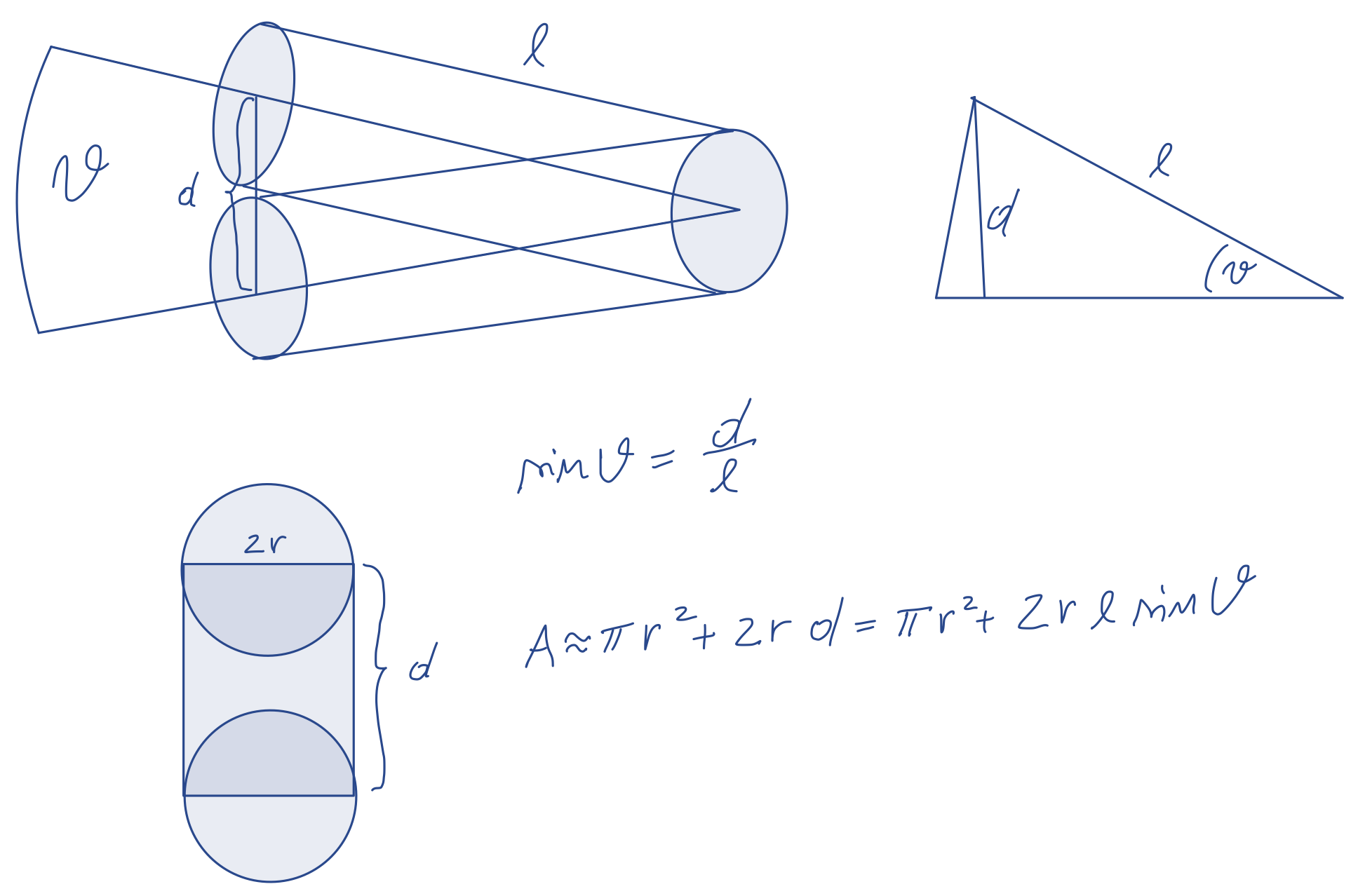
From the picture we can approximate the crossection as a function of angle to be: $$A = \pi r^2 + 2 r l \sin\theta$$
Probability for angle is distributed exponentially, hence we can write: $$P(\theta) = C e^{-\alpha \theta}$$
The normalization constant $C$ can be eliminated by requiring normalization of probability: $$1=\int_0^{\pi/2} d\theta P(\theta) = \frac{C}{\alpha}(1-e^{-\alpha \pi/2})\rightarrow C=\frac{\alpha}{1-e^{-\alpha \pi/2}}$$
Hence a closed form probability for angle is: $$P(\theta) = \frac{\alpha e^{-\alpha \theta}}{1-e^{-\alpha \pi/2}}$$
The unknown coefficient $\alpha$ can be obtained by the statement that only one in hundred million of shells turn for 90$^\circ$: $$p_0=10^{-8}=\frac{\alpha e^{-\alpha \pi/2}}{1-e^{-\alpha \pi/2}}=\frac{\alpha}{e^{\alpha \pi/2}-1}$$
Next we want to calculate the average crossection $<A>$ and its variance. The average is: $$<A> =\int_0^{\pi/2} d\theta P(\theta) (\pi r^2 + 2 r l \sin\theta)=\pi r^2 + 2r l <\sin\theta>$$ where the integral over angle $\theta$ to get $<\sin\theta>$ will need to be carried out numerically.
To get the variance, we also need: $$<A^2>=\int_0^{\pi/2} d\theta P(\theta) (\pi r^2 + 2 r l \sin\theta)^2=(\pi r^2)^2+2\pi r^2 2 r l <\sin\theta>+(2 r l)^2 <\sin^2\theta>$$
The standard deviation is the square root of the variance, i.e., $$\sigma_A = \sqrt{<A^2>-<A>^2}=2 r l \sqrt{<\sin^2\theta>-<\sin\theta>^2}$$
$$A \approx \pi r^2 + 2 r l <\sin\theta> \pm 2 r l \sqrt{<\sin^2\theta>-<\sin\theta>^2}$$The air density has maximum $\rho_{max}=1.293$ kg/m$^3$ and minimum $\rho_{min}$=1 kg/m$^3$ with the average $<\rho>=(\rho_{max}+\rho_{min})/2=1.1465$ kg/m$^3$ and $\sigma_\rho=(\rho_{max}-\rho_{min})/(2\sqrt{3})=0.0846$ kg/m$^3$, because the probability distribution is constant.
The coefficient $c$ has average $0.45$ with $\sigma_c=0.005$
We next compute $<\theta>$ and $<\theta^2>$:
from scipy.integrate import quad
from scipy.optimize import root_scalar

sr = root_scalar(lambda a: a/(exp(a*pi/2)-1)-10**-8, bracket=[0.01, 20.], method='brentq')
print(sr)
a = sr.root

def P(th):
    return a*exp(-a*th)/(1-exp(-a*pi/2))

norm=quad(lambda th: P(th),0,pi/2)[0] # checking that probability is normalized
print('Norm=', norm)
tha = quad(lambda th: sin(th)*P(th),0,pi/2)[0] # average <sin(th)>
tha2=quad(lambda th: sin(th)**2*P(th),0,pi/2)[0] # average <sin^2(th)>

print('<sin(theta)>=',tha)
print('<sin^2(theta)>',tha2)
      converged: True
           flag: 'converged'
 function_calls: 15
     iterations: 14
           root: 13.378119683088366
Norm= 1.0
<sin(theta)>= 0.07433358789414495
<sin^2(theta)> 0.010930508834082253
We are now in a position to estimate the coefficient $k$ of drag.
m=50.  # mass in kg is measured very precisely

c=ufloat(0.45,0.005) # drag coefficient is known approximately
r = 155e-3/2 # radius of 155mm shell
l = 1.       # length of the shell in m
A = ufloat(pi*r**2 + 2*r*l*tha, 2*r*l*sqrt(tha2-tha**2)) # cross-section due to finite angle

rhomax=1.293
rhomin=1.0
rho = ufloat((rhomax+rhomin)/2, (rhomax-rhomin)/(2*sqrt(3.)))

print('c=', c, 'sigma/<>=', c.std_dev/c.nominal_value)
print('A=', A, 'sigma/<>=', A.std_dev/A.nominal_value)
print('rho=', rho, 'sigma/<>=',rho.std_dev/rho.nominal_value)


ka = c*rho*A/(2*m)
print('ka=', ka)
c= 0.450+/-0.005 sigma/<>= 0.011111111111111112
A= 0.030+/-0.011 sigma/<>= 0.37496186024270517
rho= 1.15+/-0.08 sigma/<>= 0.07377393321960764
ka= 0.00016+/-0.00006
We see that the worst error is in the projectile crossection, meaning that the projectile is not very stable in the air. This is where some engeneering of the shape is necessary to improve the stability of the direction.
The second is the density of the air. Here it is hard to improve unless the missile is guided with high tech equipment, otherwise the air density is not possible to control. Of course the "aerodinamics" of the projectile could reduce $c$ substantially, which is a major goal of all realistic missile engeneering.
Next we calculate the trajectory with varying $k$ around its average value to estimate the derivative. (Note that the wrap function from module uncertainty is not working here).
We are interested in distance in lateral direction where the projectile falls ($x$ at the point $z=0$) and its error estimate.
We are thus computing $D(k)$ and we will estimate $$\sigma_D = \sigma_k \left|\frac{d D(k)}{dk}\right|$$
def dxn(t,u,k): # approproate for odeint
    """
    The derivative for projectile motion with air resistance
    """
    g = 9.82
    x,z,xdot,zdot = u
    dx = xdot
    dz = zdot
    dxdot = -k * xdot * sqrt(xdot**2+zdot**2)
    dzdot = -g -k * zdot * sqrt(xdot**2+zdot**2)
    return array([dx,dz,dxdot,dzdot])

def hit_target(t, u, k):
    # We've hit the target if the z-coordinate is 0.
    return u[1]

hit_target.terminal = True # Stop the integration when we hit the target.
hit_target.direction = -1 # We must be moving downwards (don't stop before we begin moving upwards!)

def max_height(t, u, k):
    # The maximum height is obtained when the z-velocity is zero.
    return u[3]


def odes(t0f,x0,k): # solve the ODE problem
    sol = solve_ivp(dxn, t0f, x0, dense_output=True, args=(k,),
                    events=(hit_target, max_height))
    print(sol)
    return sol.y_events[0][0,0]

# choose an initial state
v0 = 1000. # velocity magnitude in m/s
x0 = [0, 0, v0*cos(pi/4), v0*sin(pi/4)] # initial velocity at 45 degrees
t0f = (0,100)

k0=ka.nominal_value
k1=k0 + 0.2*ka.std_dev
k2=k0 - 0.2*ka.std_dev
print([k0,k1,k2])

fk = odes(t0f,x0,k0)

dfdk=(odes(t0f,x0,k1)-odes(t0f,x0,k2))/(k1-k2)

print('Distance where projectile hits=', fk)
print('Error of the distance=', abs(dfdk)*ka.std_dev)
[0.000156794235343206, 0.00016878309811701073, 0.00014480537256940127]
  message: A termination event occurred.
  success: True
   status: 1
        t: [ 0.000e+00  1.414e-06 ...  6.405e+01  6.485e+01]
        y: [[ 0.000e+00  1.000e-03 ...  1.148e+04  1.152e+04]
            [ 0.000e+00  1.000e-03 ...  1.750e+02  1.165e-12]
            [ 7.071e+02  7.071e+02 ...  5.382e+01  5.232e+01]
            [ 7.071e+02  7.071e+02 ... -2.193e+02 -2.209e+02]]
      sol: <scipy.integrate._ivp.common.OdeSolution object at 0x7f7a08e23a30>
 t_events: [array([ 6.485e+01]), array([ 2.565e+01])]
 y_events: [array([[ 1.152e+04,  1.165e-12,  5.232e+01, -2.209e+02]]), array([[ 7.557e+03,  5.378e+03,  1.610e+02, -1.421e-14]])]
     nfev: 92
     njev: 0
      nlu: 0
  message: A termination event occurred.
  success: True
   status: 1
        t: [ 0.000e+00  1.414e-06 ...  6.109e+01  6.334e+01]
        y: [[ 0.000e+00  1.000e-03 ...  1.078e+04  1.089e+04]
            [ 0.000e+00  1.000e-03 ...  4.758e+02 -4.547e-13]
            [ 7.071e+02  7.071e+02 ...  5.355e+01  4.931e+01]
            [ 7.071e+02  7.071e+02 ... -2.096e+02 -2.142e+02]]
      sol: <scipy.integrate._ivp.common.OdeSolution object at 0x7f7a09119d90>
 t_events: [array([ 6.334e+01]), array([ 2.491e+01])]
 y_events: [array([[ 1.089e+04, -4.547e-13,  4.931e+01, -2.142e+02]]), array([[ 7.174e+03,  5.134e+03,  1.555e+02,  2.842e-14]])]
     nfev: 92
     njev: 0
      nlu: 0
  message: A termination event occurred.
  success: True
   status: 1
        t: [ 0.000e+00  1.414e-06 ...  5.041e+01  6.650e+01]
        y: [[ 0.000e+00  1.000e-03 ...  1.105e+04  1.223e+04]
            [ 0.000e+00  1.000e-03 ...  3.310e+03  1.819e-12]
            [ 7.071e+02  7.071e+02 ...  9.286e+01  5.577e+01]
            [ 7.071e+02  7.071e+02 ... -1.756e+02 -2.284e+02]]
      sol: <scipy.integrate._ivp.common.OdeSolution object at 0x7f7a09151910>
 t_events: [array([ 6.650e+01]), array([ 2.646e+01])]
 y_events: [array([[ 1.223e+04,  1.819e-12,  5.577e+01, -2.284e+02]]), array([[ 7.988e+03,  5.652e+03,  1.671e+02,  1.421e-14]])]
     nfev: 86
     njev: 0
      nlu: 0
Distance where projectile hits= 11517.658105652063
Error of the distance= 3341.5938853340604
Clearly, this error is enormous. The distance is 11.5 km with a 3.3 km error. This is unacceptable even for WW1 ammunition. Hence, improving the aerodynamic shape such that the cross-sectional area is constant, and coefficient $c$ is reduced, was essential.
If we eliminate the error of the cross-section, we get an error in distance of around 870 m, which is much more realistic for classical weaponry. Of course the decrease in $c$ could further decrease the error and increase the reach.
Homework:
In addition to uncertainty in drag coefficient $k$, imagine we also have some uncertainty in the velocity $v_0$ and its lunching angle $\theta$. First let's eliminate the error in crossection area $A=\pi r^2$. Next assume that $v_0$ has still average 1000 m/s, but its distribution is triangular between 999 m/s and 1001 m/s. The angle $\theta$ is much harder to control on uneven surface under constant explosions. Assume that $\theta$ is distrbuted normally with standard deviation of 2 degrees.
How large is the error of projectile reach?